Introduction

In the world of programming, efficient algorithms play a crucial role in determining the performance of our code. One way to analyze and predict the scalability of our code is through Big O notation. Big O provides a framework for classifying algorithms based on their runtime behavior as the input size increases. I will try to explain what this is and why I think we don't need to worry about it.

Big O Algorithm Analysis

Big O notation allows us to assess how code execution time scales with the size of the data it processes. In other words, it answers the question, "How does code slow down as data grows?" Ned Batchelder, a Python developer, beautifully described this concept in his PyCon 2018 talk titled "How Code Slows as Data Grows".

To illustrate the significance of Big O, let's consider a scenario where we have a certain amount of work that takes an hour to complete. If the workload doubles, it might be tempting to assume that it would take twice as long. However, the actual runtime depends on the nature of the work being done.

For instance, reading a short book takes an hour, and reading two short books will take approximately two hours. But if we can sort alphabetically 500 books in an hour, sorting 1,000 books will likely take longer than two hours. This is because we need to find the correct place for each book in a larger collection. On the other hand, if we are simply checking if a new book fits on the shelf, the runtime remains roughly constant, regardless of the number of books.

The Big O notation precisely captures these trends in algorithmic performance. It provides a way to evaluate how an algorithm performs regardless of the specific hardware or programming language used. Big O notation does not rely on specific units like seconds or CPU cycles but focuses on the relative growth rate of an algorithm's runtime.

Big O Orders

Big O notation encompasses various orders that classify algorithms based on their scaling behavior. Here are the commonly used orders, ranging from the least to the most significant slowdown:

1. O(1), Constant Time: Algorithms that maintain a constant runtime, regardless of input size.

2. O(log n), Logarithmic Time: Algorithms with runtime proportional to the logarithm of the input size.

3. O(n), Linear Time: Algorithms with runtime proportional to the input size.

4. O(n log n), N-Log-N Time: Algorithms with runtime proportional to the input size multiplied by the logarithm of the input size.

5. O(n^2), Polynomial Time: Algorithms with runtime proportional to the square of the input size.

6. O(2^n), Exponential Time: Algorithms with exponentially growing runtime as the input size increases.

7. O(n!), Factorial Time: Algorithms with runtime proportional to the factorial of the input size (the highest order).

The notation uses a capital O followed by parentheses containing a description of the order. For example, O(n) is read as "big oh of n" or "big oh n." It's important to note that there are more Big O orders beyond the ones mentioned here, but these are the most commonly encountered ones.

Simplifying Big O Orders

Understanding the precise mathematical meanings of terms like logarithmic or polynomial is not essential for using Big O notation effectively. Here's a simplified explanation of the different orders:

• O(1) and O(log n) algorithms are considered fast.

• O(n) and O(n log n) algorithms are reasonably efficient.

• O(n^2), O(2^n), and O(n!) algorithms are slow.

While there can be exceptions to these generalizations, they serve as helpful rules of thumb in most cases. Remember that Big O notation focuses on the worst-case scenario, describing how an algorithm behaves under unfavorable conditions.

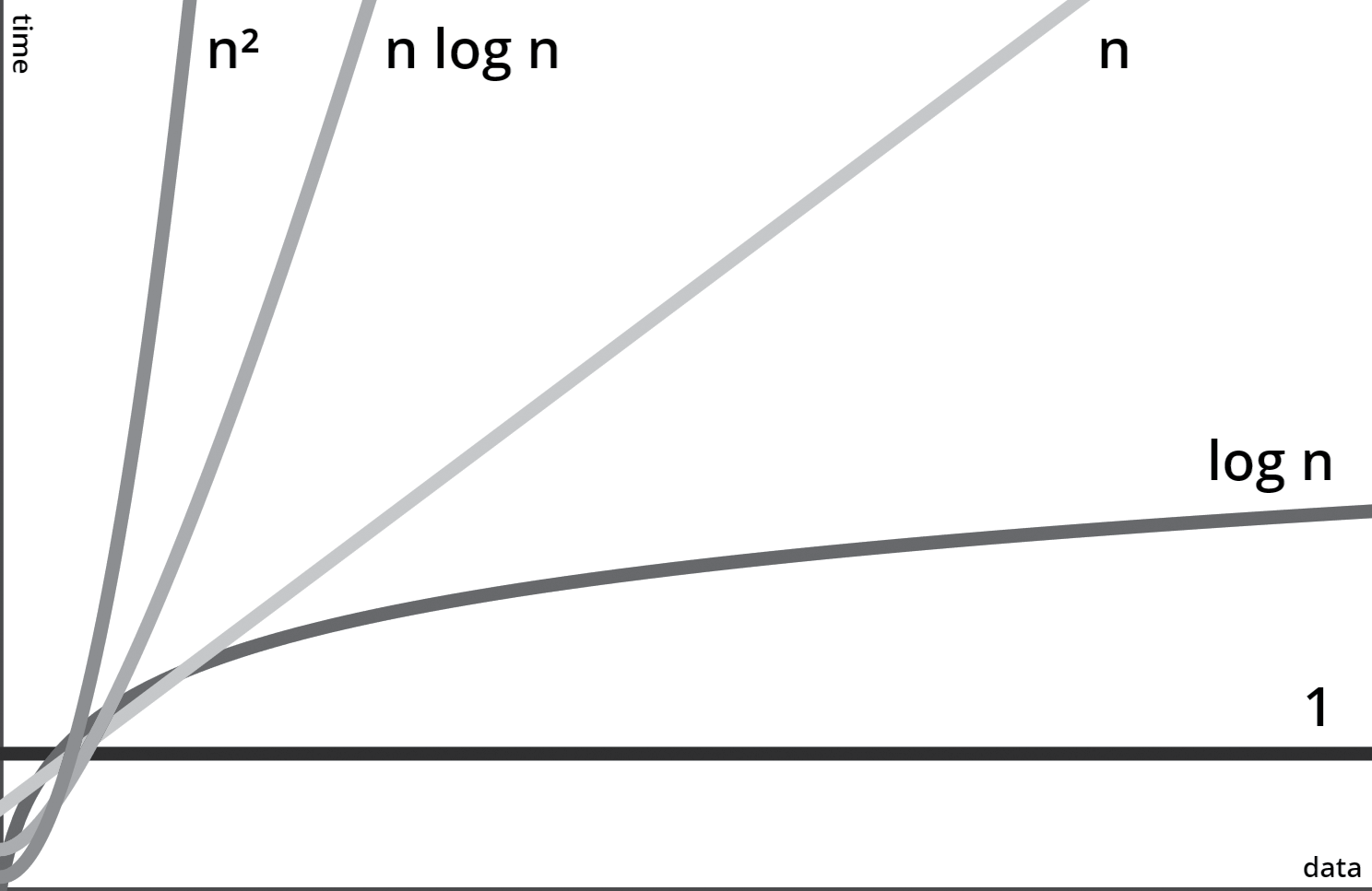
Graphically it is also very easy to appreciate:

Some examples

O(1), Constant Time

def print_first_element(lst):
    print(lst[0])

No matter how big the list is we will always take the same amount of time to get the first element.

O(log n), Logarithmic Time

def binary_search(arr, target):
    low = 0
    high = len(arr) - 1

    while low <= high:
        mid = (low + high) // 2
        if arr[mid] == target:
            return mid
        elif arr[mid] < target:
            low = mid + 1
        else:
            high = mid - 1

    return -1

This code implements the binary search algorithm, which operates on a sorted list. It repeatedly divides the search space in half until it finds the target element. The number of times we can divide any list of size n in half is log2(n) (this is simply a mathematical fact that you’d be expected to know). Thus, the while loop has a big O order of O(log n), in other words, the runtime grows logarithmically with the input size.

O(n), Linear Time

def find_max(arr):
    max_value = float('-inf')
    for num in arr:
        if num > max_value:
            max_value = num
    return max_value

This code snippet finds the maximum value in a list. It iterates through each element once, comparing it with the current maximum value. The runtime increases linearly with the input size. The more elements, the longer it takes.

O(n log n), N-Log-N Time

def binary_search(arr, target):
    low = 0
    high = len(arr) - 1
    arr.sort() # we suppose this is O(n)
    while low <= high:
        mid = (low + high) // 2
        if arr[mid] == target:
            return mid
        elif arr[mid] < target:
            low = mid + 1
        else:
            high = mid - 1

    return -1

In this example, we have the same binary search we had above but the function first sorts the input list. If we suppose that the sort operation is linear with cost O(n), then the runtime of this version of the function grows in proportion to n log n.

O(n^2), Polynomial Time

def bubble_sort(arr):
    n = len(arr)
    for i in range(n):
        for j in range(0, n - i - 1):
            if arr[j] > arr[j + 1]:
                arr[j], arr[j + 1] = arr[j + 1], arr[j]

This code snippet implements the bubble sort algorithm. It compares adjacent elements and swaps them if they are in the wrong order, repeatedly iterating over the list until it becomes sorted. The runtime increases quadratically with the input size.

O(2^n), Exponential Time

def fibonacci(n):
    if n <= 1:
        return n
    return fibonacci(n - 1) + fibonacci(n - 2)

This code calculates the Fibonacci sequence recursively. It exhibits exponential growth as the input size (n) increases because each recursive call branches into two more recursive calls, leading to a large number of redundant computations.

O(n!), Factorial Time

def permute(arr):
    if len(arr) == 0:
        return [[]]
    permutations = []
    for i in range(len(arr)):
        rest = arr[:i] + arr[i+1:]
        for p in permute(rest):
            permutations.append([arr[i]] + p)
    return permutations

This code generates all permutations of a given list. It uses a recursive approach, where it selects an element from the list and recursively generates permutations for the remaining elements. The number of permutations grows factorially with the input size.

I won't delve into further details as I believe this type of evaluation is unnecessary. Let's see why.

Considering the Size of n

While Big O notation is a powerful tool for analyzing algorithmic efficiency, it's important to remember that its significance is most apparent when dealing with a large amount of data. In real-world scenarios, the amount of data is often relatively small. In such cases, investing significant effort in designing sophisticated algorithms with lower Big O orders may not be necessary.

This is the last article in the series about optimizing and evaluating PHP applications/coreBOS performance for large datasets. I revised my knowledge of big O notation in case we could use it to evaluate some of our bottlenecks, but I understand that even with 32 million records we are still talking about small numbers for today's processing power. Our constraints are not going to be in algorithms but in business processes.

The algorithms we use and understanding big O notation will be useful to make decisions, but I am aligned with Rob Pike, the designer of the Go programming language when he expressed this idea in one of his rules of programming: "Fancy algorithms are slow when 'n' is small, and 'n' is usually small". Most developers work on everyday applications rather than massive data centers or complex computations. Profiling your code, which involves running it under a profiler, can provide more concrete insights into its performance in such contexts.

Conclusion

Understanding Big O notation and algorithm analysis empowers developers to design efficient code that can handle increasing data sizes gracefully. By classifying algorithms based on their scaling behavior, we gain insights into how different orders impact runtime. While Big O notation is most valuable when dealing with substantial data, profiling remains a practical approach for optimizing code in everyday programming tasks. By combining these techniques, developers can strike a balance between efficiency and practicality, ultimately enhancing their software's performance.

Be careful with Accidentally Quadratic code and keep security in mind!